Description
UXO Detection
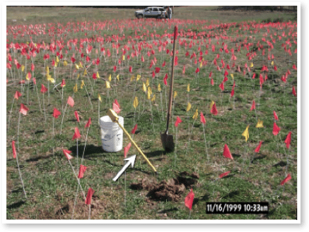
Former gunnery ranges and offshore locations in the U.S. and elsewhere contain unexploded ordnance items that were fired for target practice or improperly disposed. A traditional approach to locating such items is known as 'Mag and Flag'; where operators using crude magnetometers sweep over an area, locating anomalies by the sound the instrument makes, and placing a flag in the location of an anomaly.
Tunnel Detection and Perimeter Security
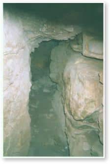
Tunnels crossing national borders or the perimeter of secure installations are another problem that can be addressed by magnetometers. The tunnels themselves are difficult to detect, but activity within the tunnels often creates or disturbs the magnetic field and can readily be detected. For this application, long arrays of magnetometers are required in order to cover the entire perimeter of an installation or along a border. Clearly, devices need to be small, low power, and less expensive for this application.
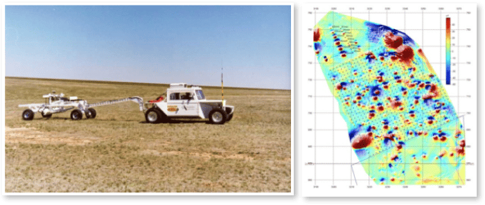
More modern is the "Digital Geophysics" method, where data is gathered over the field, stored, and later analyzed. Maps and tables are then made of the anomaly locations.
While digital geophysics provides a more accurate and comprehensive mapping of targets, its drawback is that the process takes several days. A real-time instrument could pinpoint anomalies in real time, yet be as light-weight and low-power as the simple "Mag-and-Flag" devices.
Unattended Ground Sensors
Unattended Ground Sensors are systems used by the military for monitoring purposes. Such systems may contain a camera, seismic sensors, magnetometers, and other devices to detect movement. These devices require extremely low power sensors, as they may be required to operate over a long period of time. The communications and processing systems may be of a slightly larger power consumption, as they may be placed in a sleep mode when no activity is present. The sensors themselves, however, must operate continuously, and therefore require a very low power consumption. As advances in communications and processing capabilities are made, it is envisioned that these devices could be broadcast from airborne platforms in large quantities to monitor potentially hostile territory. This would provide a market for a huge number of sensors, which would drive their production cost down.
Unmanned Vehicle Deployment
There is increasing interest in Unmanned Aerial Vehicle (UAV) platforms for carrying sensors across survey areas. Such vehicles offer the potential for high productivity, greater safety, and significantly lower cost over other survey methods. Clearly, MFAM sensors would greatly increase the practicality of UAV platforms, due to their smaller size, causing less interference with the aerodynamics of the flight platform, and their lower power requirement, greatly reducing the battery size and weight.
Eddy Current Measurement
The MFAM sensors also provide exceptional spatial and temporal resolution. We now have the technology to revolutionize magnetic sensing. Here are some examples of the amazing performance benefits of the small size of these sensors.
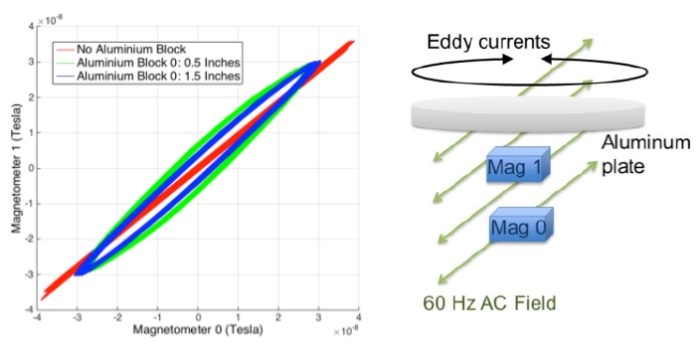
These sensors output field readings at 1000 Hz. This leads to some fascinating observations. For instance, waveforms from power lines can be fully observed and filtered, if desired, not just aliased into a lower frequency. Such aliasing typically produces strange artifacts and noise. We can even measure eddy currents in non-magnetic materials using the ever-present 60 Hz noise as a transmitter.
Changing magnetic fields induce eddy currents in conductive objects. These induced currents produce magnetic fields that are out-of-phase with the field causing them. By making measurements of the out-of-phase component of the magnetic field, we can measure the eddy current. This allows for the sensing of even non-ferrous conductors, something not typically associated with magnetometers.
The graph on the left shows the output of one sensor plotted on the horizontal axis, and the other sensor along the vertical axis. This produces Lissajous patterns according to the relative frequency and phase of the two readings. In this case the frequencies are the same, so we get a circular pattern if the two signals are perfectly out of phase, and a line if they are in phase. Elliptical patterns are the result of something in between. We can clearly see the effect as the phase difference between the two signals (caused by the eddy currents) grows larger.
Noise Cancellation in Unshielded Environments
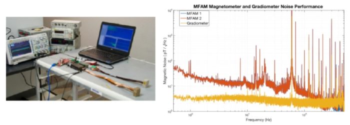
The two sensors can be positioned as close to each other as physically possible. This is made possible by the small size of the sensors and the complete absence of any cross talk between them. This close positioning allows for the measurement and subtraction of background noise to previously unheard of levels. You can reduce the background noise and make measurements to the 1 pT level, even without magnetic shielding!
Medical Applications - MCG Signal Measurement
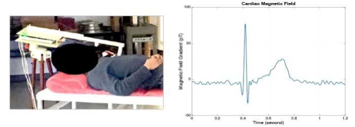
One amazing application of this is the measurement of heart MCG signals. We have demonstrated such measurements in our offices, measuring our own heartbeat signatures. By simply placing one sensor near the heart, and the other sensor on top of the first for background subtraction, magnetic fields from the heart may be measured. Better signal-to-noise ratios are obtained by stacking the data from about 100 heart beats.
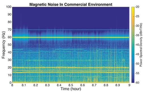
Infrastructure Monitoring
Another example of measurements that can be made in new ways with miniature total field sensors is sensing the signature of buildings and infrastructure. Buildings environments are rich in magnetic fields. These fields change with moving elevators, HVAC operations, lighting, and even moving doors and furniture. We can make a fascinating plot of the signature of a building. Plotting the FFT of a long time series of data produces virtually a building "fingerprint". Such a plot is shown below.